AStream tutorial

AStream: An R package for annotating LC/MS metabolomic data

Package downloads:

- AStream: Windows binary (AStream_1.0.zip)
- AStream: Package source (AStream_1.0.tar.gz)

Package dependencies:

The AStream package depends on the "multtest", "Biobase" and “plotrix" packages. The following R commands install them from the CRAN and Bioconductor package repositories:

source("http://www.bioconductor.org/biocLite.R")

biocLite("Biobase")

biocLite("plotrix")

biocLite("multtest")

Package example data:

The AStream package includes an example set of 3,148 features and 20 samples that can be loaded using the following command:

data(astream.data, package="AStream")

The intensities of this example data are also included in the following file: astream_data_example.xls

AStream tutorial

1.AStream Input Data

(a) Importing data from XCMS

(b) Loading user’s feature data

2.Running AStream

(a) data.norm

(b) isotope.search

(d) printresults

3.AStream output file

1. AStream Input Data

The input data for the AStream R-package can either be imported from an XCMS object or loaded as a data frame. The input data must contain the basic information from a LC/MS metabolomics analysis, that is, the mass to charge (m/z) value, the retention time and the detected intensities for each feature in each of the samples analyzed.

a) Importing data from an XCMS object

XCMS (http://masspec.scripps.edu/xcms/xcms.php) is one of the most commonly used open-source LC/MS preprocessing data software. It performs noise filtering, peak selection and nonlinear time alignment when multiple samples are analyzed. A complete review on this method and all the used parameters can be obtained either from the website (http://metlin.scripps.edu/download/xcmsPreprocess.pdf) or by typing vignette("xcmsPreprocess", package = "xcms") into R.

In order to explain how an XCMS object can be imported for an AStream analysis, we introduce here the commands required for a typical XCMS analysis. First, you should place the R working directory on the data path (when metabolomic samples are saved in different folders XCMS will treat the samples of each folder as different groups). Once the work directory has been set the typical XCMS analysis includes the following commands:

> library(xcms)

> xset <- xcmsSet(snthresh = 4)

> xset <- group(xset, minsamp = 3)

> xset <- retcor(xset, family = "s", plottype = "none", missing = 1, extra = 1)

> xset <- group(xset, bw = 10, minsamp = 3)

> xset <- fillPeaks(xset)

After running XCMS a LC/MS processed data object (i.e. xset) is created. We can now use AStream function import.xcms to import the required data from this object:

> library(AStream)

> input <- xcms.import(xset)

The resulting data object for AStream is a list with two elements:

(a) A dataframe (input$data) with rows corresponding to the total number of features (n=3,153 features in this case) and the first two columns indicating the m/z values (first column) and retention times (second column). The remaining columns contain the detected feature intensities for each individual, where the column names correspond to the sample names (ID).

(b) A list (input$class) that contains the group/status of each sample.

b) Loading user’s feature data

Although XCMS processing is highly recommended, users with their own feature dataset obtained using any other analysis platform can also load their data in order to perform an AStream data curation. In this case is only necessary to format the data as an R list containing the two objects required by AStream as defined previously. An example of this type of input can be directly loaded from the AStream package. This example data consists of 20 LC/MS metabolomic samples randomly divided into two groups (G1 and G2) with a total set of 3,148 features peaks:

> library(AStream)

> data(astream.data,package="AStream")

> input$data[1:3,1:6]

mzmed rtmed G1_1 G1_2 G1_3 G1_4

1 61.027944319865 426.307329158435 106306.455097724 127154.336715698 96099.2742362155 110844.540377937

2 64.0163388523736 389.533531615442 469463.71550916 462603.441696861 468016.930060338 470743.191450544

3 65.0190493567312 389.697081910654 19129.1374828996 17687.7633235852 16159.3797389168 16819.0124880034

> input$class[1:22,1]

> input$class

class

1 G1

2 G1

3 G1

4 G1

5 G1

6 G1

7 G1

8 G1

9 G1

10 G1

11 G2

12 G2

13 G2

14 G2

15 G2

16 G2

17 G2

18 G2

19 G2

20 G2

2. Running AStream

a) data.norm()

Once AStream data has been loaded to the defined workspace, we can start the analysis by calling the first function data.norm which performs outlier detection and feature selection based both on the retention time differences and on the pairwise intensity correlation of all the feature pairs. This function has five parameters:

· std.outliers (default=3): This parameter is used to fix the threshold value for the outlier detection method. Samples having a standardized outlier score over this value will be excluded for further analysis. We can also turn off outlier detection by setting std.outliers=0.

· zero.missing (default=TRUE): Logical value, when TRUE intensity values equal to zero are considered as missing values.

· min.corr (default=0.75): Correlation threshold. Feature pairs with a pairwise intensity correlation below this value will be excluded.

· max.rt (default=3): Retention time difference threshold. Feature pairs with a retention time difference over this value will be excluded.

· fplot (default=TRUE): Logical, if TRUE summary figures are plotted.

The following two examples show how to perform a default analysis and an analysis modifying several input. Relevant information on the analysis is displayed on the R prompt such as the number of samples excluded and the number of feature pairs selected:

EXAMPLE 1: Default analysis data.norm	EXAMPLE 2: Modified parameters data.norm
> feat1 <- data.norm(input) DATASET: - #Features: 3148 - #Samples: 20 - RT limits: [ 1.6 , 1795.95 ] - M/Z limits: [ 61.03 , 998.78 ] NORMALIZATION BY FEATURE MEDIAN... OUTLIER DETECTION... - Max Dev allowed=3 - SAMPLE #5 (G1_5) excluded: [3.929815,-2.897018] COMPUTING CORRELATION MATRIX... - Zeros = Missing 0% 10% 20% 30% 40% 50% 60% 70% 80% 90% 100% FEATURE PAIRS SELECTION RESULTS: - MAX RT DIFFERENCE ALLOWED: 3 - MIN CORRELATION ALLOWED: 0.75 - FEATURE PAIRS SELECTED: 11317 > names(feat1) [1] "data" "class" "mz" "rt" "feature.set" "outliers" "scores"	> feat2 <- data.norm(input, max.rt = 2.5, min.corr = 0.60) DATASET: - #Features: 3148 - #Samples: 20 - RT limits: [ 1.6 , 1795.95 ] - M/Z limits: [ 61.03 , 998.78 ] NORMALIZATION BY FEATURE MEDIAN... OUTLIER DETECTION... - Max Dev allowed=3 - SAMPLE #5 (G1_5) excluded: [3.929815,-1.568823] COMPUTING CORRELATION MATRIX... - Zeros = Missing 0% 10% 20% 30% 40% 50% 60% 70% 80% 90% 100% FEATURE PAIRS SELECTION RESULTS: - MAX RT DIFFERENCE ALLOWED: 2.5 - MIN CORRELATION ALLOWED: 0.6 - FEATURE PAIRS SELECTED: 18005 > names(feat2) [1] "data" "class" "mz" "rt" "feature.set" "outliers" "scores"
EXAMPLE 1 SUMMARY PLOT

EXAMPLE 2 SUMMARY PLOT

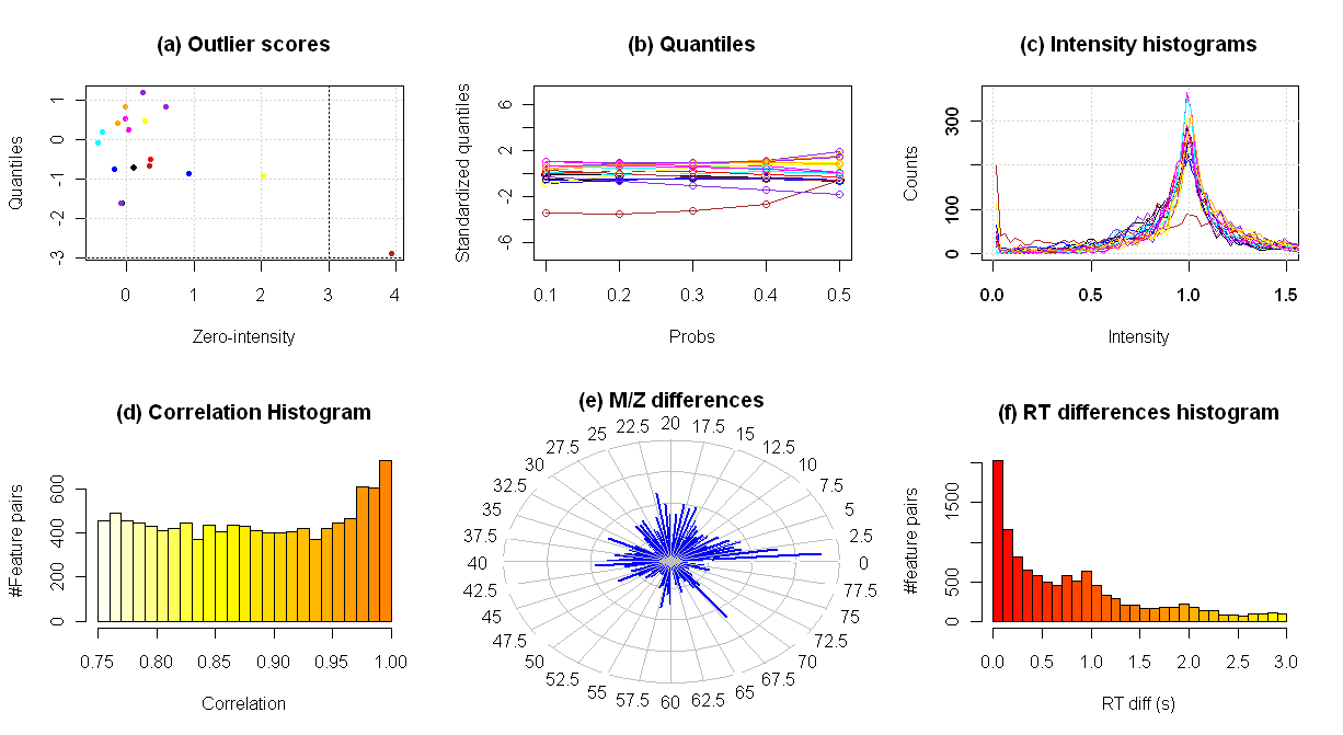
The plots that are generated can be very useful to understand normalization and outlier exclusion process. Looking to the following example, the plots show the following information:

(a) Outlier scores of each sample: The scores computed from the number of features having zero intensity are represented over the x-axis, while the scores computed from the intensity quantiles are represented over the y-axis. In our example, one sample is excluded because it zero-intensity score (x-axis) is greater than the default score threshold std.outliers=3 (bottom-right orange point).

(b) Computed intensity quantiles (10%, 20%, 30%, 40% and 50%) for each sample. Each quantile has been standardized using the values of all the samples.

(c) Normalized intensity distributions of each sample. This figure also helps to detect the outlier sample (orange) having a very high value at intensity 0 and a low value at intensity 1.

(d) Histogram of the pairwise feature intensity correlation values that are greater than the specified threshold (i.e. 0.75 in example 1 and 0.60 in example 2). We can observe the inflation within the values near to 1 due to the existence of isotopes and adducts highly correlated.

(e) Polar histogram of the m/z differences within the selected feature pairs. The peaks due to ¹²C-¹³C isotopes (m/z_diff=1.0033), [M+H]-[M+Na] adducts (m/z_diff=21.982) and [M+H]-[M+NaHCOOH] adducts (m/z_diff=67.987) are clearly visible.

(f) Histogram of the retention time differences that are greater than the specified threshold (i.e. 3.0 in example 1 and 2.5 in example 2). We can observe the inflation within the values near to 0 due to the existence of isotopes and adducts with almost the same retention time values.

Once data.norm function has been executed, the generated output list consists of all the necessary data for the isotope and adduct search analysis:

· data: Numeric matrix with the intensities of all the features (rows) from all samples (columns). In the present example, there are n=19 final samples after excluding one sample having an outlying signal profile.

> dim(feat1$data)

[1] 3148 19

· class: Group label of each included sample.

> feat1$class[,1]

[1] "G1" "G1" "G1" "G1" "G1" "G1" "G1" "G1" "G1" "G1" "G2" "G2" "G2" "G2" "G2" "G2" "G2" "G2" "G2" "G2"

· rt and mz: Retention time and m/z values of each feature.

· feature.set: Set of feature pairs that will be analyzed in order to find isotopes, adducts or fragments. This set contains all the pairs that have passed the correlation and retention time filter thresholds specified in data.norm.

> feat1$feature.set[1:10,]

Index feature 1 Index feature 2 Correlation %samples RTdiff M/Zdiff

[1,] 1 35 0.7722203 100 1.16187443 23.019208

[2,] 1 153 0.7765506 100 0.96656101 60.024970

[3,] 2 97 0.8418388 100 0.25841026 41.026011

[4,] 2 195 0.8360164 100 1.84080403 67.986864

[5,] 2 542 0.7992878 100 0.91842920 135.981157

[6,] 4 5 0.8114268 100 0.01603013 0.988777

[7,] 4 11 0.9074511 100 0.00960247 6.509211

[8,] 4 14 0.8939059 100 0.02002257 7.508971

[9,] 4 113 0.7943203 100 0.18891644 40.972375

[10,] 4 115 0.7504487 100 0.20864333 42.987411

· outliers: Indexes of the outlier excluded samples within the initial sample group.

· scores: Outlier scores of each sample within the initial sample group. Two scores are provided, the first corresponding to the number of features with zero intensity and, the second, corresponding to the intensity quantiles. In the present example, the scores corresponding to the outlier sample (sample #5) have been highlighted. The outlying values from this sample are indicative of a potential problem either in the sample collection phase or during the LC/MS data acquisition process:

> feat1$scores

$int_0

[1] 0.11228042 -0.17964868 0.26947301 -0.13473651 3.92981477 0.24701693 -0.42666560 -0.02245608 -0.02245608

[10] 0.58385819 -0.06736825 0.35929735 0.92069946 2.02104760 -0.22456084 0.33684127 -0.08982434 -0.35929735

[19] 0.02245608 -0.13473651

$int_1

[1] -0.7257414 -0.7654592 0.4761860 0.1038420 -2.8970182 1.1807430 -0.1038420 0.5233418 0.8306186 0.8248309

[11] -1.6179217 -0.5120058 -0.8800208 -0.9313024 0.1438316 -0.6664879 -1.6177946 0.1941364 0.2443339 0.4189088

b) isotope.search()

The following step in the analysis is to search for isotopes within the feature pairs selected by data.norm. The function isotope.search performs this search by grouping all those features that fulfill the expected m/z differences between carbon isotopes of the same molecular compound:

· 1st ¹³C-isotope peak difference: m/z[¹³M] - m/z[¹²M] = 1.0033

· 2nd ¹³C isotope peak difference: 2*(m/z[¹³M] - m/z[¹²M]) = 2.0066

isotope.search function has three input parameters:

· ftlist: Dataset list as returned by data.norm.

· mz.tol (default=3e-3): Tolerance for m/z values.

||m/z[feature_i] - m/z[feature_j]| - 1.0033| < mz.tol à features i and j will be grouped as ¹²C-monoisotopic peak and first ¹³C-isotope peak of the same molecular compound

||m/z[feature_i] - m/z[feature_j]| - 2.0066| < mz.tol à features i and j will be grouped as ¹²C-monoisotopic peak and second ¹³C-isotope peak of the same molecular compound

· fplot (default=TRUE): Logical, if TRUE summary figures are plotted.

The output of this function is the same than the input F but with an added “isotopes” component which contains the obtained information relative to isotopes. In the present example:

EXAMPLE 1: isotope.search

> feat1 <- isotope.search(feat1, mz.tol = 3e-3)

PE ANALYSIS:

- M/Z tolerance: 0.003u

- C12-isotope m/z: 12u

- C13#1-isotope m/z: 13.00335u

- C13#2-isotope m/z: 14.0067u

- 13C#1/12C-isotope: 378 feature pairs

- 13C#2/12C-isotope: 71 feature pairs

- Total number: 449 isotope patterns

> feat1$isotopes[1:10,]

Index-12C Index-13C1 Index-13C2 Intensity-12C Intensity-13C1 Intensity-13C2

[1,] 12 16 0 3090537.8 130994.89 0.00

[2,] 13 17 0 1079753.1 44512.43 0.00

[3,] 23 25 0 175807.6 25626.86 0.00

[4,] 39 46 0 272485.3 19822.19 0.00

[5,] 41 47 0 654658.6 41185.92 0.00

[6,] 42 48 0 1151918.4 66914.15 0.00

[7,] 45 52 0 460785.7 43766.34 0.00

[8,] 86 88 0 514900.2 10721.60 0.00

[9,] 98 102 0 1796847.8 85156.37 0.00

[10,] 98 0 108 1796847.8 0.00 26828.69

EXAMPLE 1 SUMMARY PLOT

In the present example, feat1$isotopes contains the isotope grouping results with the feature indexes linked to the obtained isotope patterns. The summary plot shows the mean intensity ratios between first and second ¹³C-isotopic peaks and ¹²C–monoisotopic peak. Given the lower abundance of C13 species, the detected patterns must have intensity ratios lower than 1 as the abundances (intensities) of ¹³C isotopes are further lower than ¹²C isotopes.

c) adduct.search()

The adduct.search function performs the last data reduction step of the AStream analysis. The input parameters are:

· ftlist: Dataset list as returned by isotope.search.

· mz.tol (default=3e-3): Tolerance for m/z differences.

· adducts (default=0): According to the particular technical parameters of the LC/MS acquisition process, the user can define its own set of adducts to perform the adduct search step. This must be a data.frame object with two columns, the first indicating the adduct mass and the second the corresponding label. The protonated compound (i.e. [M+H]), is the reference adduct and therefore must always be present in this data frame. By default, if no data.frame object is used, a predefined set of adducts will be used (see below).

· onlyIsotopes (default=TRUE): If True, the adduct search will only take into account those features that have been previously associated to an isotope pattern. This option is highly recommended for robustness in metabolite annotation.

· fplot (default=TRUE): Logical, if TRUE summary figures are plotted.

Two examples are showed below, the first one with the default set of adducts and the second using an alternative set of adducts loaded using the “adducts” argument.

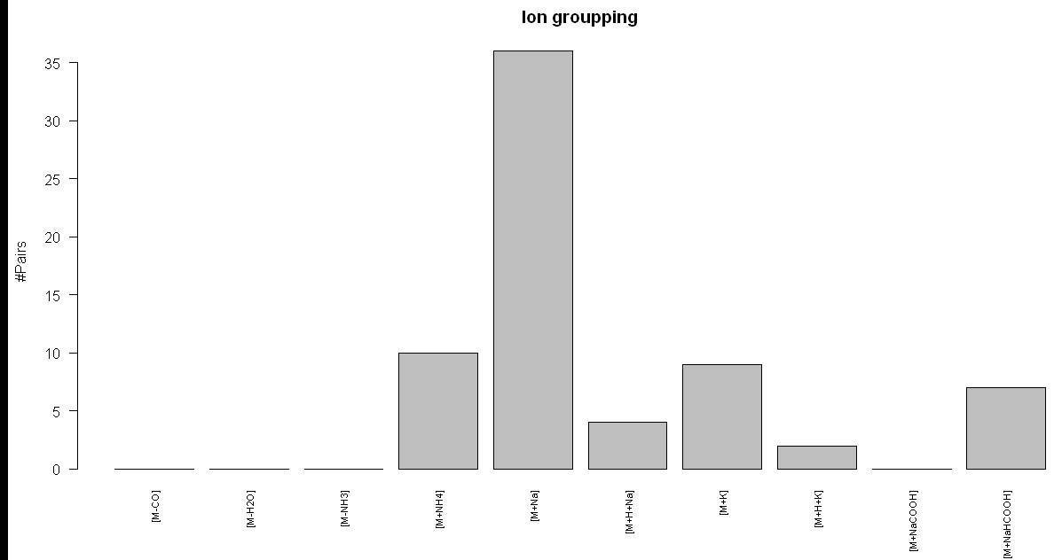
EXAMPLE 1: adduct.search

> res <- adduct.search(feat1)

ADDUCT ANALYSIS:

- M/Z tolerance: +/-0.003u

- 0 [M-CO]adducts.

- 0 [M-H2O]adducts.

- 0 [M-NH3]adducts.

- 10 [M+NH4]adducts.

- 36 [M+Na]adducts.

- 4 [M+H+Na]adducts.

- 9 [M+K]adducts.

- 2 [M+H+K]adducts.

- 0 [M+NaCOOH]adducts.

- 7 [M+NaHCOOH]adducts.

EXAMPLE 2: adduct.search

> adductlist <- data.frame(cbind(c(1.007276, 18.033823,22.989218,38.963158,68.99472),

+ c("[M+H]","[M+NH4]","[M+Na]","[M+K]","[M+NaHCOOH]")))

> adductlist

X1 X2

1 1.007276 [M+H]

2 18.033823 [M+NH4]

3 22.989218 [M+Na]

4 38.963158 [M+K]

5 68.99472 [M+NaHCOOH]

> res2 <- adduct.search(feat1, adducts=adductlist)

ADDUCT ANALYSIS:

- M/Z tolerance: +/-0.003u

- 10 [M+NH4]adducts.

- 36 [M+Na]adducts.

- 9 [M+K]adducts.

- 7 [M+NaHCOOH]adducts.

> res2[1:20,]

C12isotope C13#1 isotope C13#1 ratio C13#2 isotope C13#2ratio [M+NH4] [M+Na] [M+K] [M+NaHCOOH]

[1,] 12 16 0.04238579 0 0.00000000 0 0 0 0

[2,] 13 17 0.04122463 0 0.00000000 0 0 0 0

[3,] 23 25 0.14576649 0 0.00000000 0 0 0 0

[4,] 39 46 0.07274591 0 0.00000000 0 0 0 0

[5,] 41 47 0.06291206 0 0.00000000 0 0 0 0

[6,] 42 48 0.05808931 0 0.00000000 0 0 0 0

[7,] 45 52 0.09498200 0 0.00000000 0 0 0 0

[8,] 86 88 0.02082268 0 0.00000000 0 0 0 0

[9,] 98 102 0.04739209 108 0.01493098 0 0 0 0

[10,] 99 103 0.04784580 0 0.00000000 0 171 0 0

[11,] 102 108 0.31505204 0 0.00000000 0 0 0 0

[12,] 115 117 0.18524925 0 0.00000000 0 0 0 0

[13,] 138 140 0.05027759 0 0.00000000 0 0 0 0

[14,] 144 148 0.05115318 0 0.00000000 0 0 0 0

[15,] 145 149 0.05692672 0 0.00000000 0 0 0 0

[16,] 146 150 0.05210245 0 0.00000000 0 0 0 0

[17,] 158 161 0.04571414 163 0.01947436 246 261 339 0

[18,] 161 163 0.42600300 0 0.00000000 0 0 0 0

[19,] 184 192 0.06698323 0 0.00000000 0 0 0 0

[20,] 185 193 0.06751841 0 0.00000000 0 292 0 0

The output of this function is a list of feature groups that can be definitively related to a single compound. For each compound (row) the indexes of the related features corresponding to isotopes and adducts are given in the successive columns. If we want to visualize all the features that have been related to a specific compound we can call the function plotcompound using the compound index in the adduct.search output (i.e. res). Here we show the distribution of two different detected compounds (#10, #71) obtained from the previous analysis:

EXAMPLE: plotcompound

> res[10,]

C12isotope C13#1 isotope C13#1 ratio C13#2 isotope C13#2ratio [M-CO] [M-H2O] [M-NH3] [M+NH4] [M+Na] [M+H+Na] 99 103 0.0478458 0 0.0 0 0 0 0 171 0

> plotcompound(10, feat1, res)

> res[71,]

C12isotope C13#1 isotope C13#1 ratio C13#2 isotope C13#2ratio [M-CO] [M-H2O] [M-NH3] [M+NH4] [M+Na] [M+H+Na] 733 741 0.1313409 0 0.0 0 0 0 831 856 0

> plotcompound(71, feat1, res)

d) printresults()

After applying AStream’s analysis flow, the non-redundant and robust set of metabolic features can be exported as a tab delimited text file using the printresults function. This table summarizes the principal characteristics of each compound an provides a direct link to the METLIN metabolomics database (http://metlin.scripps.edu/metabo_search.php).The input parameters for this function are:

· filename: name of the file where the results will be extracted.

· ftlist: Output returned by isotope.search.

· results: Output returned by adduct.search.

· range (default = 1e-2): m/z tolerance for the search in the Metlin database.

· Mzsort (default = FALSE ): If TRUE results will be sorted by m/z value. If FALSE, results will be sorted by P-Value if there are two groups of samples.

In the present example, the output file can be generated as it follows:

EXAMPLE: printresults

> printresults("results.txt", feat1, res)

3. AStream Output Files

The tab delimited text file where the results are extracted using the printresults function has the following fields. Example values are referred to the example line below:

· IndexFeature: Index within the original feature set (AStream input) of the feature labeled as [M+H]⁺ (i.e. 486).

· MassSubmitted: Expected m/z value of the compound [M] ([M+H]⁺- [H]) (i.e. 188.1045).

· M/Z: m/z value of the feature labeled as [M+H]⁺ (i.e. 189.1121).

· RT: retention time value of the feature labeled as [M+H]⁺ (i.e. 1050.36).

· P-Value: If two groups of samples have been provided, P-Value of the intensity association test between those groups (i.e. 0.00625).

· FoldChange: If two groups of samples have been provided, intensity fold change between those groups (i.e. 3.57).

· N1: If two groups of samples have been provided, number of samples of the first group having non zero intensity at the feature labeled as [M+H]⁺ (i.e. 9).

· N2: If two groups of samples have been provided, number of samples of the second group having non zero intensity at the feature labeled as [M+H]⁺ (i.e. 10).

· Metlin: Link to the Metlin database (i.e. http://metlin.scripps.edu/metabo_list.php?mass_min=188.0945&mass_max=188.1145).

· 13C#1-isotope: If the 13C-isotope feature has been identified this field contains 4 numbers separated by a space corresponding to the index of the 13C-isotope within the original feature set, the intensity ratio between 13C-isotope and 12C-isotope features, the pairwise intensity correlation of those features and their retention time difference (i.e. 495 0.1 1 0.208).

· 13C#2-isotope: If the 14C-isotope feature has been identified this field contains 4 numbers separated by a space corresponding to the index of the 14C-isotope within the original feature set, the intensity ratio between 14C-isotope and 14C-isotope features, the pairwise intensity correlation of those features and their retention time difference (i.e. NA).

· Adducts: If there are one or more adduct features identified, they are listed here giving their label and their index within the initial feature set (i.e. [M+NH4]:573 [M+Na]:597).

· NFG: Number of features grouped within this compound (i.e. 4).

Example line in the present example:

IndexFeature

MassSubmitted

M/Z

P-value

FoldChange

Metlin

13C-isotope

14C-isotope

Adducts

NFG

486

188.1045

189.1121

1050.36

0.00625

3.57

http://metlin.scripps.edu/metabo_list.php?mass_min=188.0945&mass_max=188.1145

495 0.1 1 0.208

[M+NH4]:573 [M+Na]:597

MID	Mass	Name	MS/MS	Structure
3800	188.10486	3-Methylsuberic acid Formula: C₉H₁₆O₄ CAS : 34284-35-0	NO